The signal you leave behind
When training data are scarce relative to the number of features, a predictor can rely heavily on a few strong signals. Selecting only those features may discard complementary information. Feeding everything into a single model does not guarantee that weaker signals will be used effectively either.
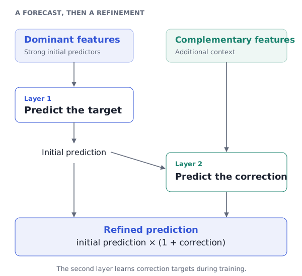
HEFS gives different feature groups distinct roles. The first model makes a prediction. The next learns how complementary information should adjust it. This is particularly relevant for non-stationary time series, where the relationships that matter can change.
01 / PREDICT
Start with dominant features
Use domain knowledge or a training-set relevance score to form the first group. Train an initial predictor on those features.
02 / LEARN TO REFINE
Make room for the others
Search for useful scaling corrections during training. A second model learns them from complementary features and the first prediction.
03 / COMBINE
Apply a learned correction
At inference, multiply the first prediction by one plus the predicted correction. No observed test target is needed.
What the experiments show
The paper compares LightGBM-based methods on a synthetic dataset, M4 Yearly, and Weather. The two-layer HEFS model has the lowest reported test error on Synthetic and M4, and ties backward selection on Weather at the published precision.
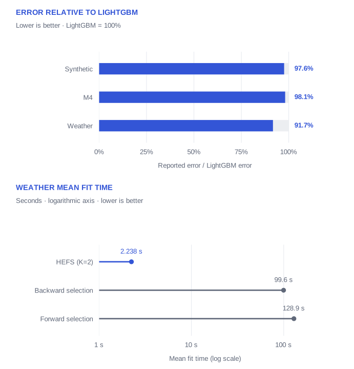
On Weather, HEFS has the same displayed test error as backward selection, with a reported mean fit time of 2.238 s versus 99.60 s. The advantage is not universal: three layers do not consistently improve test error, and benefits may diminish with abundant data or no clear feature-group structure.
Explore the results and metric note →
A small hierarchy, an explicit objective
The key connection between layers is a cost-optimization block: it searches for a scaling correction that minimizes a chosen final loss, then uses that correction as a training target. This search does not require differentiating the final loss. The supplied implementation uses LightGBM learners and absolute-error correction search.
HEFS organizes how features are used; it does not simply return one selected subset. The estimator expects the columns to be arranged into groups before fitting.
Cite this work
Published in Digital Signal Processing, volume 168, article 105528 (2026); available online August 2025. Publisher / DOI.
@article{karaca2026hefs,
  title   = {Hierarchical ensemble-based feature selection for time series prediction},
  author  = {Karaca, Huseyin and Tumay, Aysin and Koc, Ali Taha and Kozat, Suleyman Serdar},
  journal = {Digital Signal Processing},
  volume  = {168},
  pages   = {105528},
  year    = {2026},
  doi     = {10.1016/j.dsp.2025.105528},
  url     = {https://doi.org/10.1016/j.dsp.2025.105528}
}